DOSY on Bruker Avance III
this tutorial is copy from Operating DOSY Experiments, and make some minor changes.
In Topspin, go to Help -> Manuals, find “DOSY” handout. Read and understand the principle.
Decide a suitable d20 (big delta), typical range 0.01s to T1[shortest], and p30[litter delta], typical range 0.5 to 3ms. note for cryoprobe p30 <= 2ms, and critical to prevent gradient duty cycle p30/(d1+aq)<5%.
lock; shim; atma; rga. if your sample is high salt water sample, make sure you have correct 90 pulse, for normal sample the default 90 pulse is Ok; make the suit d1 ( 2s-5 x T1 is better); and aq need be long enough to provide good resolution. T1 estimation can ref here.
Run a spectrum. This one is with gpz6 = 2 (default; means 2% of the gradient amp power is used).
Create a new expriment by "iexpno" or "edc" choose “Use current parameters“. Don’t do rga. type gpz6 and enter 95 (give the gradient amp 95% of the power). run the expriment.
5a. If the tall peaks have negative spikes on their sides that cannot be fixed by phase correction, type loopadj, then rerun the expriments.
compare the two spectra with 2% and 95% gradient powers. if the latter is less than 1% of of the former, you need to reduce d20. If the latter is greater than 10% of the former, you need to increase d20. d20 could range from 0.02 s to 0.5 s. every time you change d20, you need to rerun both expriments. normally, 5% or 2% is OK.
Once an optimal d20 is decided, create another new file by choosing DIFFUSION2D. change d20 to the value that you have determined. enter a suitable NS (should be multiple of 16). enter command dosy 2 95 16 q y y. This is a macro that will run a 2D DOSY expt. Meaning of the parameters: 2: beginning gradient amplitude = 2%; 95: ending gradient amplitude = 95%; 16: number of 1d slices = 16; q: increment is square rooted (alternatively, you could do l for linear increment); the first y: begin acquisition; the second y: do a rga before the run. For more details, please read the Bruker brochure mentioned in step 1.
when done, click ProcPars tab and change SI of F1 column to 64. In command line, type xf2 to Fourier transform (only in the 2nd dimension). Correct phase. Read Bruker manual to learn how to phase a 2D spectrum. Only phase-correct rows.
type setdiffparm. This sends the exprimental parameters that you used to Dynamics Center for data fitting.
on main menu, click Analysis -> T1/T2 module -> Dynamics Center. Follow the flow in the new window. Instruction on using Dynamics Center can be found here.
there are other reference DOSY/Diffusion on Avance III, Operating DOSY Experiments, and Setting up Dosy expriments.
Gradient strengths calibrations
1. Calibrate by a phantom sample
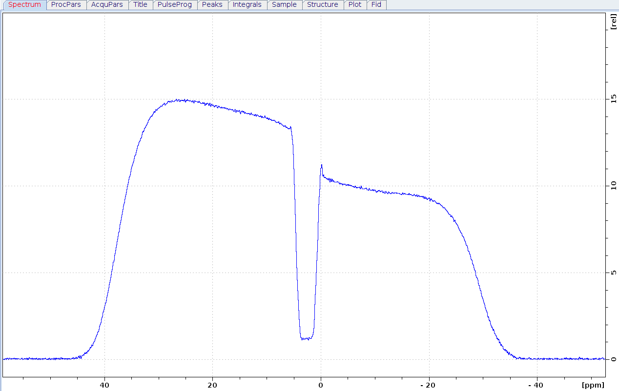
The profile expriment seems to be more direct and accurate for measuring the gradient strength, but there exist two problem.
One is difficult to make one precise thinness phantom sample in NMR tube. Below I make two phantom tube, one is 1mm thin of Teflon, and one is ~3mm thin unkown plastic. the 1mm one is too thin to keep level, so recommended thinness 2~4mm.
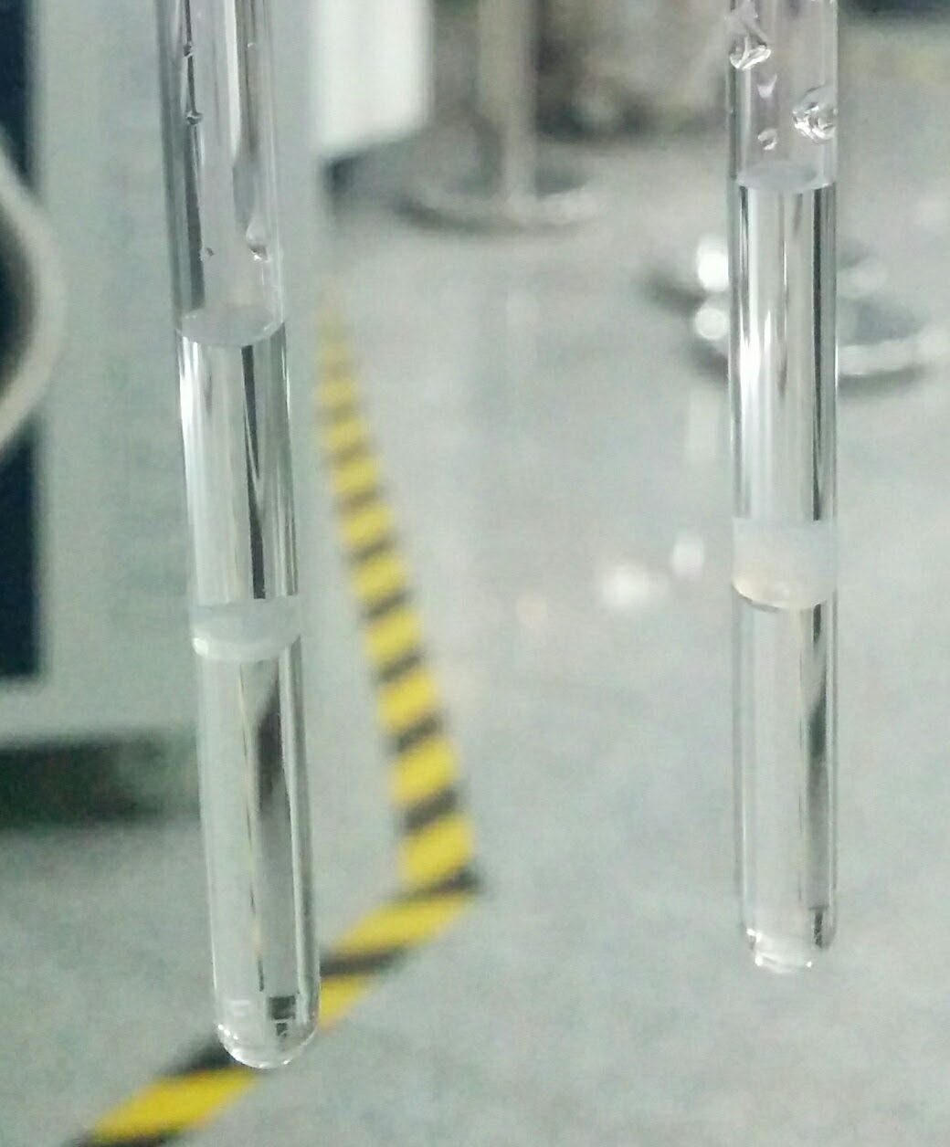
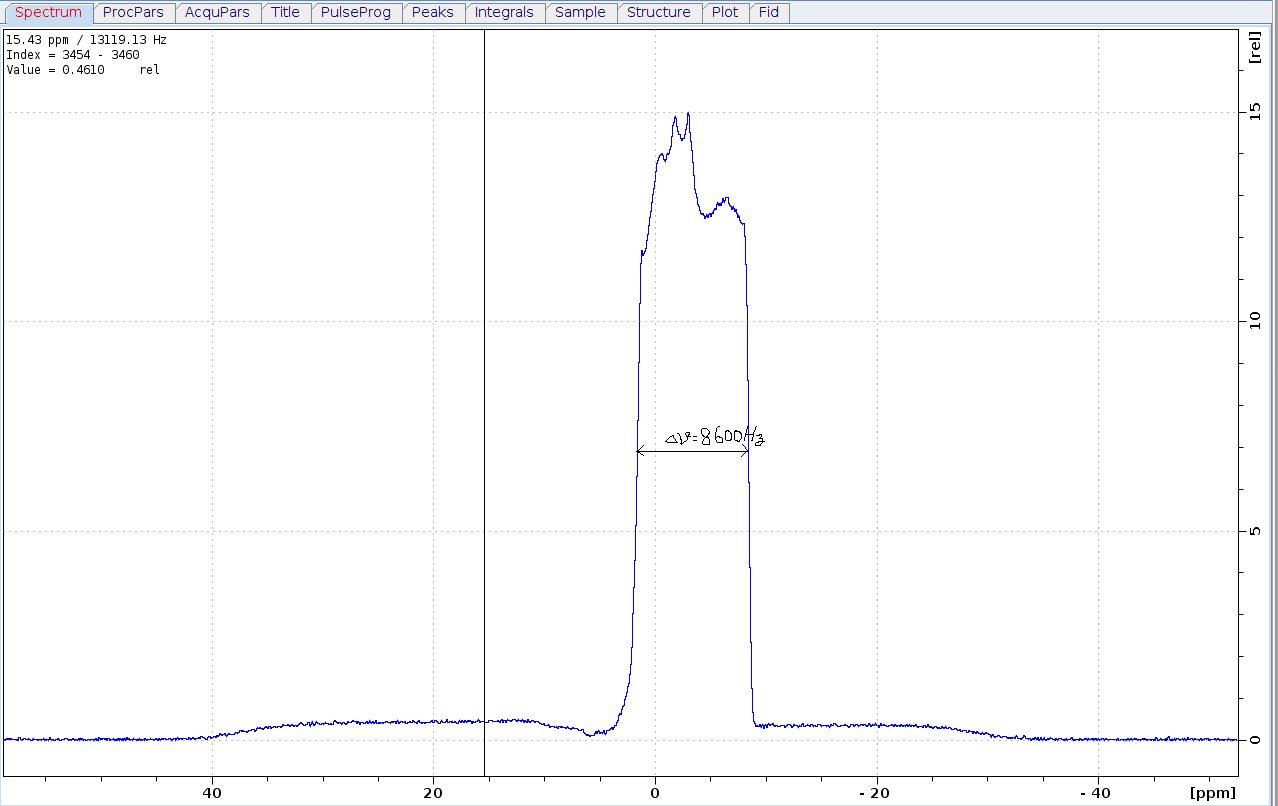
Preform the "calibgp" in bruker using 10% and 20% gradient strength. Also the dip is not sharp, and you can not get accurate how wide of the dip in gradient profile specturm. In 1mm tube there is tilted phantom, the image profile has fuzzy boundary. and the 3mm unkown plastic has nmr signal diffrent with water, so there is one platform in image profile spectrum. This method about the measurement of a 1D image profile is detailly discipted in Timothy D.W. Claridge's Book, using the width 8600Hz and 0.33cm height of the phantom, the maximum gradient strength for 850MHz/AvanceIII/CPTXI system is 59.78 G/cm. Because the unkown plastic is out of shape after insert to nmr tube, and the width of dip is not precise, this strength is approximate value.
Another problem is that the applied gradient strenth in the profile expriment is steady, but PFG-NMR sequence which use in diffusion menasure will count the eddy currents induced by gradient pulse. So the calibrated gradient strength that is found from a profile expriment is less than that from a diffusion expriment using known diffusion coefficient sample[1].
[1]: Artefacts and pitfalls in diffusion measurements by NMR, Magn. Reson. Chem. 2002; 40: S139–S146, DOI: 10.1002/mrc.1112
2. Calibrate by D2O sample
This approach is susceptible on the temperature and sample. The recommended reference sample is HDO in 99.9% D2O solvent which the diffusion coefficient at 298K is 1.91 x 10⁻⁹m2s-1. 0.1% CuSO4 is added to make the peak FWHM > 3Hz.
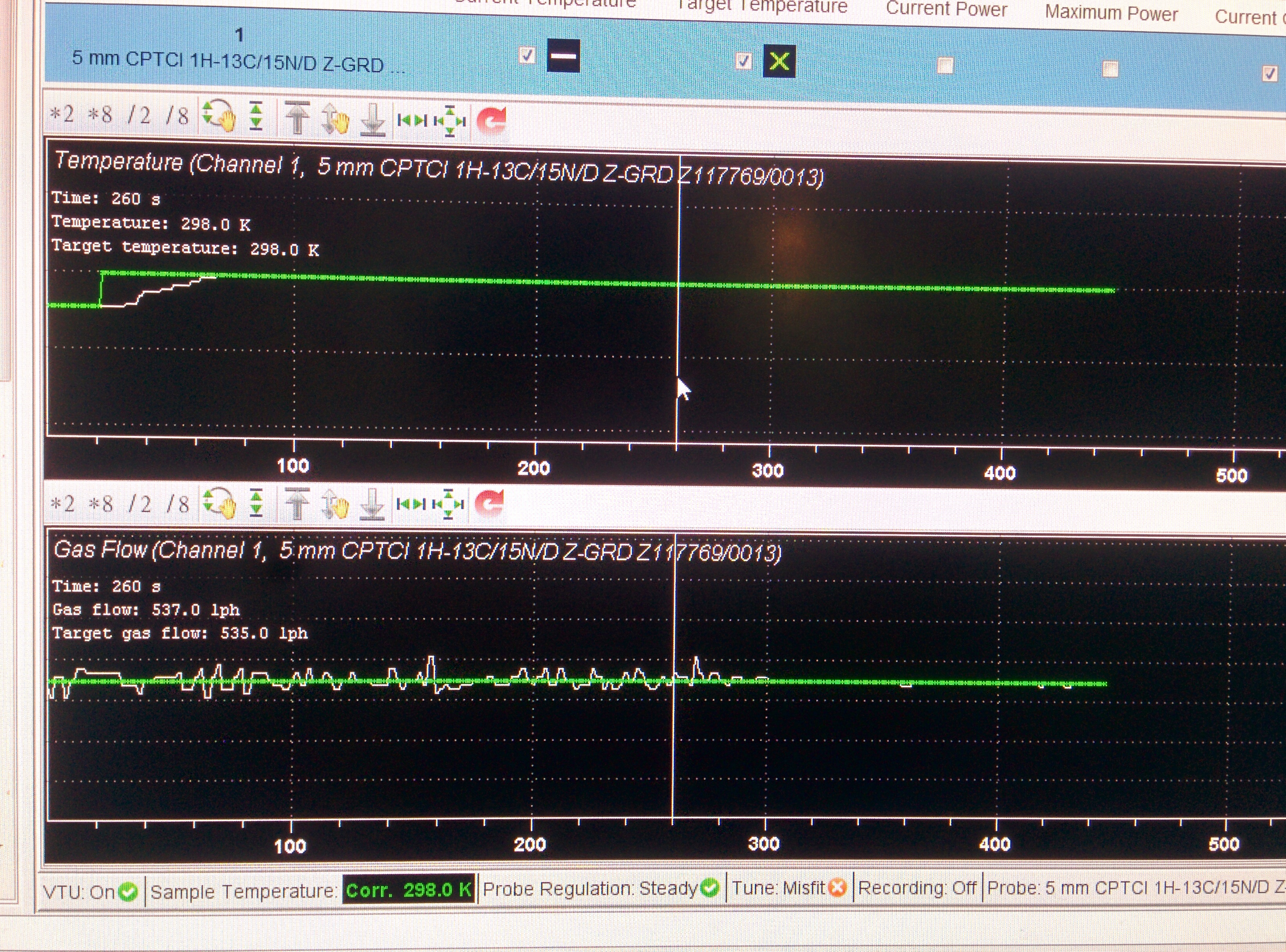
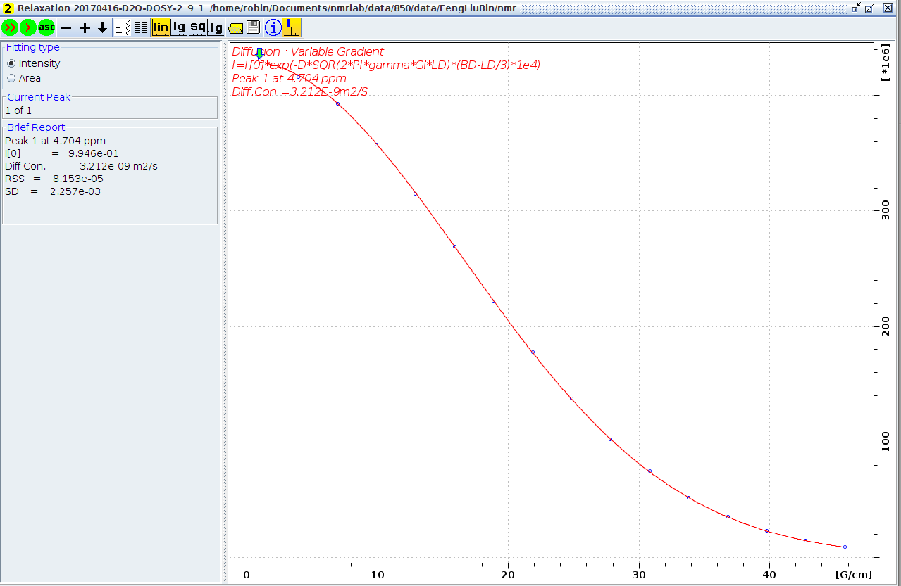
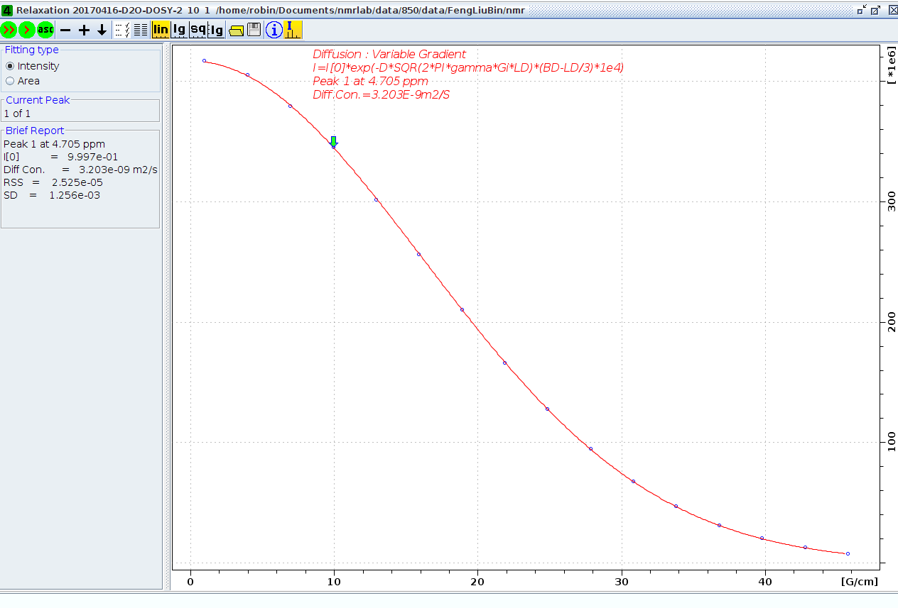
Methods: the expriment is on 850MHz Bruker Avance III system with CPTXI probe. The sample temperature is corrected by MeOD sample, and set the temperature to 298K, wait the temperature and gas flow steady 20 minutes.
note: the 90 pulse length is very important for salt water
The "ledbpgp" and "dstebpgp" expriments are carried out, and get the same result 3.2 X 10⁻⁹m2s-1, and now the system set the gradient strength 53.5 G/cm in "setdiffparm", from Gnew = sqrt(D/Dliter) X Gold equation given the system gradient strength 69.3 G/cm. This value is not far off the strength 59.78 G/cm from the profile expriment. As described above, this value is more accurate.
Diffusion coefficient measurement
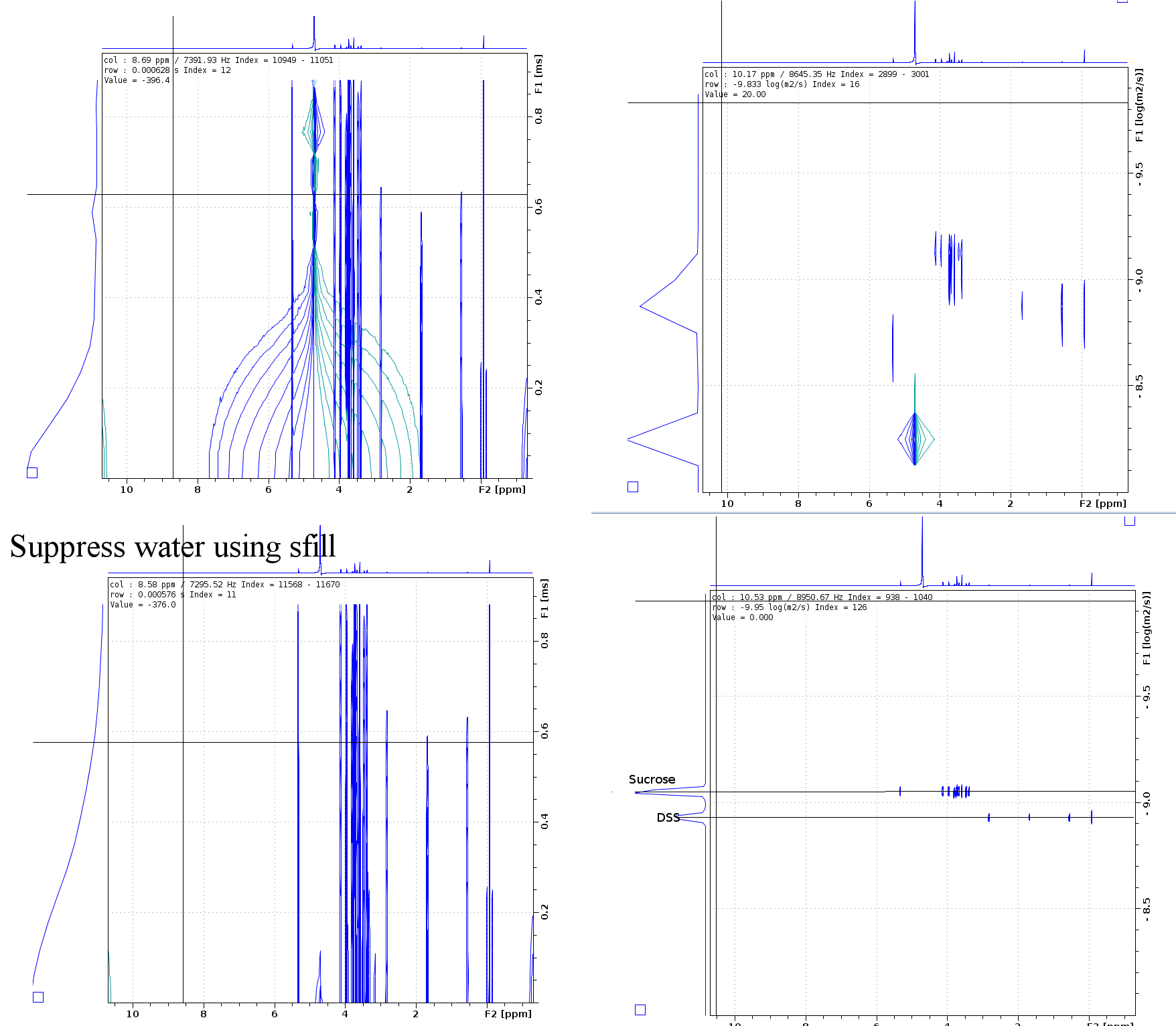
Sample info: 2mM Sucrose 0.5mM DSS 2mM NaN3 10%D2O 90%H2O
Pulse sequence: ledbpgppr2s with pr water suppression
Methods: the expriment is on 850MHz Bruker Avance III system with CPTXI probe. Temperature is set 298K, wait the temperature and gas flow steady 20 minutes.
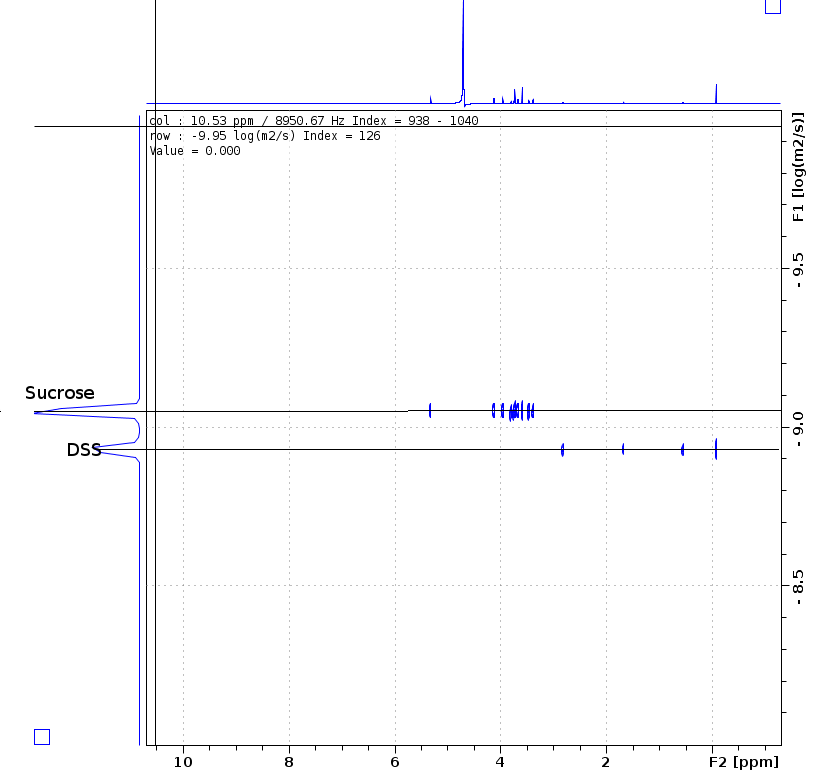
note: post-process using "sfill" deduct the water signal is very important when not good water suppression, and you can using SI(F1) more than TD(F1) to get better specturm.